


July 23, 2024 On Tuesday, July 23rd, C2SMARTER’s NYU contingent...
Read MoreAs researchers looking to address real-world questions, data is the foundation of everything. Unfortunately, high-quality, multifaceted data is often unavailable, so researchers must be resourceful. Different data sources can be fused together to create the desired richness. By interpolating new points, dataset sizes can increase while remaining faithful to the underlying truths. There is a tradeoff to be mindful of: micro-level data points will not map precisely to the real world, but when properly implemented, the broader trends will hold. For example, our project created a synthetic population of freight trucks traveling through New York City [1]. Each modeled truck has a pickup location, several drop-off locations, and carries a specific type of freight, just as real trucks would. While likely no one synthetic truck directly mirrors one in the real-world, the modeled patterns of freight movement resemble the measured patterns at the neighborhood or borough level. This article will lay out how we go from the starting assumptions to a validated model.
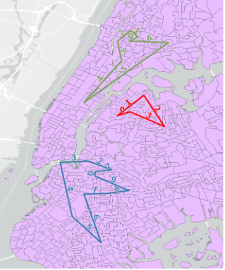
To create the synthetic freight truck population, we had to first estimate the amount of freight created and delivered (aka produced and attracted) throughout the city. This process was relatively straightforward as previous research had established relationships between each business type and size and its freight demand. However, properly distributing that freight from producers to consumers required innovation. To begin with, urban freight distribution is built on the idea of tour-based behaviors: a truck picks up its payload and then delivers it to several stops throughout the day before returning to the depot. Figure 1 has some sample tours. Trucks start at leg 0 and work their way through their routes. Building a model of citywide freight distribution required us to construct a lot of possible truck tours and then assign the right number of trucks to take each tour. Creating the right truck flows is very involved; there are roughly 350,000 trucks to assign, and tours can range in length from 3 stops up to 15 stops depending on the industry.
Because reliably finding the single best solution is not even thought possible, mathematicians have created a range of methods designed to find very good solutions. When transportation systems researchers decide which algorithm to use certain elements are considered: what data are available to input? what outputs are we looking to verify? how long are we willing to let the computer take to find an answer? what approaches have other people used to tackle similar problems? Our freight truck distribution model employed Entropy Maximization which draws inspiration from statistical mechanics, a branch of physics. Faithfully borrowing concepts from other fields is a fascinating and exciting part of transportation research for me. There is an intellectual joy in seeing the patterns of the universe repeat in unexpected places [2].
These crossovers aren’t just fascinating, but useful too. Successfully showing that the same math applies allows us to build an analogy to carry over our problem-solving intuitions. First, we need to understand entropy maximization. We can think of this process as trying to pick the most probable outcome. Dice rolls are a great illustrative example of this. We can use two six-sided dice, labeled A and B. We’ll roll both and then sum them. Table 1 displays the outcomes.

Table 1. Dice Roll Micro and Mesostate
Looking at Table 1, we can see that the mesostate of sum 7 is the most probable because there are 6 different possible microstates which could comprise it. When you abstract out details from the microstate, you arrive at a mesostate. Because of this reduction in specificity, some of the mesostates will be the same. For example, [A:2, B:3] produces the same mesostate as [A:1, B:4] even though all the individual dice rolls are different. The mesostate that entropy maximization picks will be the one which the greatest number of microstates can be generalized into. Put another way, when comparing all the mesostates you created from your microstates, pick the one which happens the most. Sometimes you need to be more specific about your mesostate though. For example, you might want the most probable outcome that is also divisible by 3. This constraint reduces your possibilities down to [3,6,9,12] with 6 now being selected.
Let’s see how much intuition we can carry over from statistical mechanics to transportation. We are now trying to select the most probable distribution of freight trucks. The question then is how to define ‘most probable.’ To do that we must first define our mesostates and microstates. In this context, the microstate is the most granular description of every possible route by single trucks owned by every company, while the mesostate is the number of trucks traveling between zones and what they are carrying. Therefore, we want to find the distribution of freight truck flow between zones that could contain the greatest number of combinations of unique trucks. Not every possible combination is valid; we determine considerations like the total amount of freight picked must equal the total amount of freight dropped off. Constraints like this help to ensure that the outcome picked by the math matches the real world.
An entropy maximization model solution method for a problem of this size (all the freight trucks in NYC) was not known to exist prior to this work, so we had to design and implement a new solution method capable of crunching our numbers. Instead of trying to satisfy all the constraints at once, it iteratively updated the amount of truck assigned to each route according to one constraint at a time. This balancing act was repeated until it settled on a solution. The output from this process is a set of tours which specify where the truck picks up freight and where that freight is being dropped off, example in Figure 1. Adding in other synthetic details, such as starting time and how many trucks are taking that route, forms the synthetic freight population. Unsurprisingly, these details had to be cobbled together from a variety of sources. Start times are based around NYC DOT bridge reports [3]. Travel times are based around the now decommissioned Uber Movement dataset [4]. Vehicle emissions were calculated based upon work from previous researchers [5]. Tying together all these data sources in a single location makes our model incredibly valuable to researchers because it allows us to study the complex relationships between the various components.
To validate our model, we calculated the roads that every truck would take in its tour and then counted how many trucks would cross the boundary between boroughs on major bridges and roads. We chose to look at the movement between boroughs for three reasons:
- 1) it was a city-wide threshold with consistent data
- 2) it matched the level of predicting power of our model
- 3) NYC DOT had quantified truck movements similarly in a recent report [6]
When we validated our model for the first time, our results were poor. We combed through every stage of the data and modeling process trying to find errors or sources of improvement. Inspiration struck with the idea of changing how we generated our truck tours.
Originally, a hypothetical tour could deliver to multiple locations spread across all five boroughs because the stops were chosen purely at random. In retrospect, this assumption is faulty because it suggested an unrealistic travel behavior. Real world carriers purposely cluster their delivery locations for efficiency reasons. This revelation led to the introduction of a distance penalty factor. Now when the algorithm was picking drop-off locations, it would be more likely to those that were close to the starting point. After this change, our results drastically improved. However, there was further potential for refinement. Our model still overestimated the number of trips traveling between Manhattan and Brooklyn or Queens. We added an additional Manhattan-specific distance penalty to reflect the ways in which the road network disincentivizes interborough trips, and the business density in Manhattan allows for greater trip clustering than in the other boroughs. This additional factor further shrank the gap between how many trips were predicted and how many were measured.
After working out a few kinks, the model proved sufficient; its predictions agree with previous work which estimated the total number of freight trucks in New York City [7] and its predictions line up well with real world observations.
This work set out to develop a model of freight truck movement across New York City. To build this deep and novel insight, we had to fuse public datasets to estimate how much freight is needed and then design a model which could allocate the demand across the city. The model design was shaped by its requirements and inspired by other fields. Importantly, a solution would not have been possible without this heterogeneity. Combining the disparate datasets, mathematical constructs, and team members’ perspectives created something far better. After an initial round of observations, our assumptions about how tours are constructed had to be altered and then further refined. With these improvements capturing real-world behavior that we were previously missing, our results became meaningfully closer to the ground truth. These iterative stages of data gathering, modeling, combination, and validation are very common in the transportation field and in the research community at large. Hopefully, this article, and the others like them [8], help to demystify them.
Footnotes
- For more about this work, you can watch the presentation or read the full report.
- Another good crossover from physics to transportation is the phenomenon of traffic shockwaves: The same math that explains sound traveling through a medium also explains groups of cars slowing down and speeding up as they travel together on the interstate.
- NYCDOT (2018). 2016 New York City Bridges and Tunnels Annual Condition Report. New York City Department of Transportation. Retrieved form https://www.nyc.gov/html/dot/downloads/pdf/dot_bridgereport16.pdf.
- Uber Movement. (2022). Available: https://movement.uber.com/?lang=en-US [Accessed 06/10/22]
- Bigazzi, A. Y., & Figliozzi, M. A. (2013). Role of Heavy-Duty Freight Vehicles in Reducing Emissions on Congested Freeways with Elastic Travel Demand Functions. Transportation Research Record 2340(1), 84–94.
- NYCDOT (2021). Delivering New York, A Smart Truck Management Plan for New York City. New York City Department of Transportation. Retrieved form https://www1.nyc.gov/html/dot/downloads/pdf/smart-truck-management-plan.pdf
- Holguín-Veras, J., Lawson, C., Wang, C., Jaller, M., González-Calderón, C., Campbell, S., Kalahashti, L., Wojtowicz, J., & Ramirez-Ríos, D. (2017). Using commodity flow survey microdata and other establishment data to estimate the generation of freight, freight trips, and service trips: guidebook (No. Project NCFRP-25 (01)).
- This article is part of a series intended to bring research by the BUILT Lab at C2SMARTER to a wider audience. The other entries are Using MATSim-NYC to Optimize the Brooklyn Bus Network Redesign and Modeling Amazon HQ2
Related Posts

ITS-NY 31st Annual Meeting and Technology Exhibition
June 13-14, 2024, Saratoga Springs, NY On June 13-14, 2024,...
Read More
SUBMIT A PROPOSAL FOR C2SMARTER’S 2024-25 RFP
C2SMARTER is soliciting proposals from its consortium faculty for research...
Read More
C2SMARTER at Smart City Expo 2024
May 22-23, 2024 C2SMARTER had the pleasure of hosting 3...
Read MoreShare
Facebook
Twitter
LinkedIn
Email
Print
Reddit